Consider a self-driving car approaching a crowded intersection. In that moment, the AI model integrated into the car processes multiple video frames. Out of hundreds of video frames, a pedestrian might appear in only a few. If the model predicts “no pedestrian” for every frame, it would still achieve about 99.9% accuracy. On paper, the model looks nearly perfect. But missing even one frame can have serious consequences.
This reflects a common challenge related to machine learning and vision classification models. For instance, an image classification model analyzes images and estimates the likelihood that a given image represents a specific object or event.
Whether detecting pedestrians in video, identifying defects in images, or flagging abnormalities in medical scans, classification models assign each input to a discrete category, such as “pedestrian” versus “no pedestrian” or “defect” versus “no defect”, by applying decision thresholds to probabilistic outputs under uncertainty.
When building and evaluating classification models, it isn’t enough to know how often a model is right. We also need to understand how it works and, more importantly, how it fails. For this reason, evaluating classification models requires more than metrics like accuracy. Classification metrics such as true positives, precision, and the F1 score reveal how and why a model succeeds or fails.
In this article, we’ll explore different classification metrics and how to validate classification models more effectively.
To evaluate classification models beyond accuracy, we can use classification metrics that compare model predictions with ground-truth labels. These are the correct labels provided by human annotations or verified data. These metrics help us understand where a model makes correct decisions and where it goes wrong. We’ll start with the most fundamental one: the true positive.
In any classification task, a model’s prediction is compared with the actual outcome to determine whether it is correct or incorrect. A true positive occurs when a model predicts positive, and the actual outcome is indeed positive.In computer vision, this includes correctly detecting a pedestrian in a video frame, identifying a defect on a manufactured part, or flagging an abnormal region in a medical scan. In each case, the model successfully identifies a positive instance that actually exists in the real world.
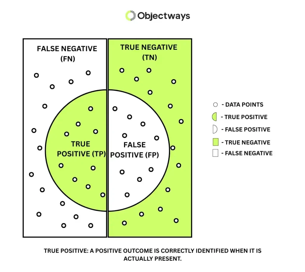
Understanding What a True Positive Is
True positives represent the moments when a model gets the most important decisions right. They often correspond to the outcomes a system is explicitly built to detect. However, maximizing true positives alone can make the model unreliable. Understanding true positives is the first step toward balancing model performance, which requires considering all possible prediction outcomes together in the confusion matrix.
A confusion matrix is the foundation for evaluating classification models. It provides a clear, structured way to understand how a model’s predictions compare with actual outcomes. Along with true positives, nearly every classification metric used to evaluate classification models is derived from the confusion matrix.
At its core, a confusion matrix compares a model’s predicted labels with the true labels. For binary yes-or-no classification problems, the confusion matrix is a 2×2 table that captures all four possible outcomes.
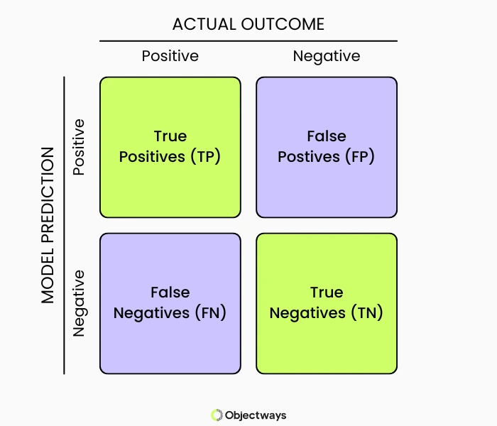
An Example of a Typical Confusion Matrix
Here’s a look at the four outcomes:
Each outcome represents a different type of success or failure. Together, they describe the complete behavior of a classification model.
Using the four possible outcomes, the confusion matrix is organized as a 2×2 table. One axis represents the actual outcome, while the other represents the model’s prediction. By counting how many predictions fall into each cell, we can gain a clear and transparent view of where the model performs well and where it struggles.
Nearly all classification metrics are derived from the confusion matrix. For example, the true positive rate, also known as recall, measures the proportion of actual positive cases correctly identified. Precision measures the proportion of predicted positives that are correct, while the F1 score balances precision and recall. We’ll explore each of these metrics in more detail next.
The true positive rate (TPR), also known as recall, measures how effectively a model identifies actual positive cases. It shows, out of all truly positive instances, how many the model correctly detects. In some domains, it is also referred to as sensitivity, but in machine learning and computer vision research, recall is the more commonly used term.
The true positive rate is calculated using two values from the confusion matrix: true positives and false negatives. It compares the number of correctly detected positive cases to the total number of actual positive cases. A model that identifies most real positives achieves high recall, whereas a model that misses many positives has low recall.
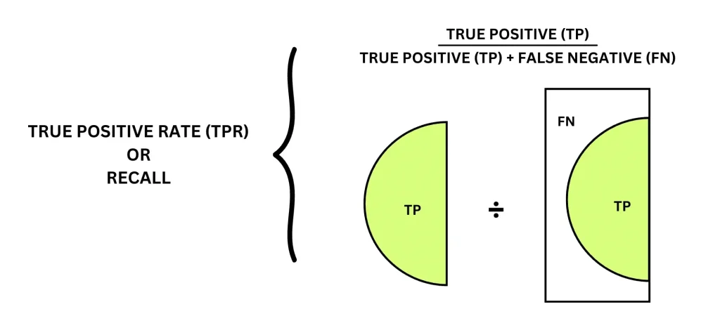
True Positive Rate or Recall Formula
Recall is important in computer vision systems where missing a positive instance can have serious consequences. Research on vision detection models highlights recall as a key metric for evaluating detection performance, particularly in scenarios involving rare or safety-critical objects.
In applications such as autonomous driving, medical imaging, and industrial inspection, models are often designed to prioritize recall to ensure that critical objects are detected, even if this results in more false positives that can be handled downstream.
Precision measures how reliable a model’s positive predictions are. It is calculated from the confusion matrix using true positives and false positives. It compares the number of correctly predicted positive instances to the total number of instances predicted as positive.
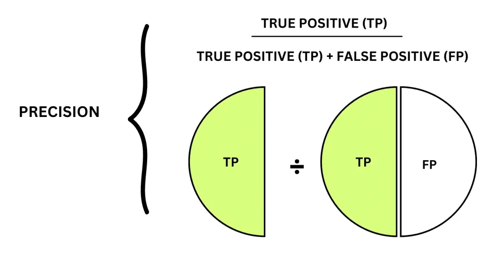
Precision Formula
When most predicted positives are correct, precision is high. When many predicted positives are incorrect, precision decreases. Precision is important in scenarios where false positives are costly or disruptive.
In computer vision systems such as facial recognition, access control, or automated quality inspection, incorrectly flagging a normal case can lead to unnecessary delays or compliance issues. In these settings, models are often tuned to favor precision so that positive predictions can be trusted, even if it means missing some true positives.
So far, we have seen what precision and recall (TPR) are and how they evaluate a model’s performance. The F1 score combines these two metrics. While precision focuses on avoiding false positives and recall focuses on avoiding false negatives, the F1 score evaluates how effectively a model performs on both at the same time.
The F1 score is the harmonic mean of the precision and recall. Because of this, the F1 score penalizes models that perform well on only one of the two metrics, making it sensitive to imbalances between precision and recall.
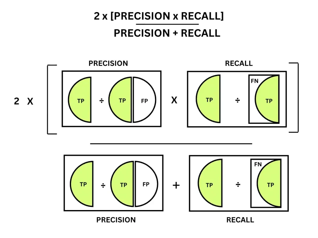
F1 Score Formula
A confidence threshold is the certainty or probability score a model assigns to a prediction, indicating how strongly it believes an instance belongs to a positive class. When this threshold is adjusted, the model’s classification behavior changes.
Predictions with confidence scores above the threshold are labeled as positive, while those below it are labeled as negative. As a result, shifting the threshold directly affects classification metrics.
The F1 score is usually computed at a single confidence threshold, but a model’s performance varies as that threshold changes. An F1 confidence curve illustrates how the F1 score evolves across different threshold values. Because most classification models output probability scores, modifying the threshold changes which predictions count as positive, also altering both precision and recall.
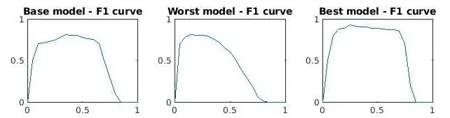
Examples of Different F1 Curves (Source)
Precision and recall typically move in opposite directions. Increasing the threshold often improves precision but reduces recall, while lowering it increases recall but may decrease precision. The F1 score reaches its maximum at the point where precision and recall are best balanced, and then declines as the trade-off between them becomes more pronounced.
Beyond classification, the F1 score is particularly valuable in tasks where both false positives and false negatives are important, such as object detection and anomaly detection. An F1 confidence curve extends this insight by helping practitioners identify the threshold that produces the strongest balance between precision and recall and by enabling more meaningful comparisons between models.
One limitation of the F1 score is that it doesn’t account for true negatives. In many real-world computer vision applications, correctly identifying negative instances is also essential. For this reason, the F1 score should be considered alongside additional classification metrics to obtain a comprehensive understanding of model performance.
A calibration curve evaluates how well a model’s predicted probabilities reflect real-world outcomes. It measures how reliable the model’s confidence scores are.
Typically, a calibration curve consists of three elements. The horizontal axis represents the model’s predicted probabilities, the vertical axis shows the observed accuracy, and the diagonal line represents perfect calibration
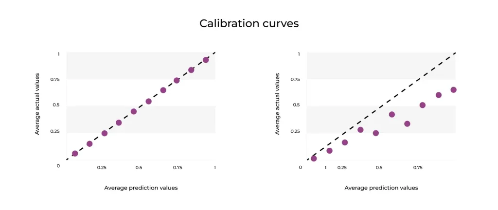
Calibration Curves for a Perfect Model Vs Overconfident Model (Source)
A perfectly calibrated model follows a diagonal line, where predicted confidence matches actual correctness. Curves below the diagonal indicate overconfidence, meaning the model assigns probabilities higher than those observed in reality, while curves above the diagonal indicate underconfidence, where the model is correct more often than its confidence suggests.
Calibration curves are especially important in high-stakes domains where probability estimates directly influence decisions. In areas such as healthcare and autonomous systems, poorly calibrated predictions can lead to incorrect risk assessments and unsafe decisions, even when overall classification performance appears strong.
Next, we’ll look at how true positive rate, precision, F1 score, and calibration curves work together in real-world model evaluation. Each classification metric tells part of the story, but not the whole story.
Recall or true positive rate indicates how effectively a model captures positive cases, especially when missed detections are costly. Precision reflects how reliable the model’s positive predictions are and helps limit unnecessary or expensive actions caused by false positives.
The F1 score combines these two metrics, providing a balanced measure when both missed detections and false positives matter. Calibration adds another layer by ensuring that predicted confidence scores align with reality.
In real-world applications, these classification metrics are evaluated together to understand how the model performs well and how it behaves under different operating conditions. This holistic view enables teams to choose appropriate thresholds, manage risk, and deploy models that align with industry-specific requirements.
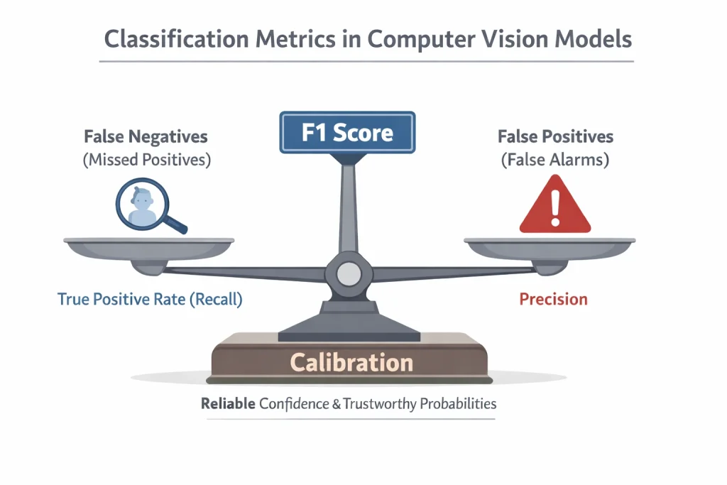
Classification Metrics Explained
Classification models fail when evaluation doesn’t reflect real-world behavior. Classification metrics such as true positive rate, precision, F1 score, and calibration are essential for understanding how models perform under real-world operating conditions, where errors have real costs.
However, meaningful evaluation depends on more than just choosing the right metrics. Models must be tested on representative, high-quality data that reflects real deployment scenarios, edge cases, and class imbalances. Without reliable annotations and evaluation-ready datasets, even well-chosen metrics can give a misleading picture of performance.
At Objectways, we help AI teams train and evaluate models using high-quality data, expert annotations, and evaluation-ready datasets designed for real-world deployment. Contact us to learn how we can support your next AI project.
Classification metrics are more than just numbers. They shape how AI and classification models are built for industry-specific applications.
Looking beyond surface-level classification metrics, the confusion matrix reveals how different errors affect model behavior, while the trade-off between recall and precision clarifies the practical costs of those errors. The key takeaway is that better classification metrics lead to better decisions, and better decisions lead to more trustworthy AI.
The four common classification tasks are binary classification, multiclass classification, multilabel classification, and ordinal classification. These classifications differ in how many labels or categories a model can predict.


Learn about the difference between machine learning vs. deep learning vs. computer vision and how these technologies work together to build smarter AI systems.

Join us as we explore what is content moderation, how platforms apply it across multimedia, and how AI and human reviewers keep online spaces safe.